 Streaming Learning Center Where Streaming Professionals Learn to Excel


Related Articles

You think you know RD Curves. You think you know encoding ladders. I’m here to tell you, you don’t know diddly.
The RD Curve above compares encoding ladders for VP9, HEVC, and H.264. It’s a short, idiosyncratic clip. Don’t focus on what you know about codec efficiencies. Focus on what you think the RD Curves tell you.
Which codec is more efficient? Easy, right? Without question, VP9. But will the VP9 ladder save you bandwidth as configured or cost you more? What about quality? More or less than H.264?
How will that change if your primary audience connects over high-bitrate connections and retrieves the top two or three rungs? What if it’s primarily a mobile audience retrieving middle-to bottom-tier content?
More importantly, what does this all mean for how you should configure your encoding ladders for advanced codecs like VP9, AV1, and HEVC?
You think you know encoding ladders, but you don’t know diddly. Take a seat, and have a listen.
Getting Started
Too much drama? Yeah, probably. Sorry. I just spent yet another day debugging a software program called the Streaming Learning Center Bitrate Explorer, or SBE. As you’ll see, building RD-Curves and BD-Rate functions is straightforward. Building algorithms to help understand them is a bear.
Here’s what I mean. Figure 2 shows the BD-Rate stats that correspond with Figure 1. These make sense. For this short clip, VP9 proves most efficient, HEVC the least efficient, and H.264 in the middle. It’s a short test clip; it happens. But the numbers clearly match the BD-Rate curves. VP9 is in green at the top, H.264 in blue in the middle, and HEVC in red at the bottom.

By definition, BD-Rate stats are the average values for all the common data points in the clips. But we don’t ship averages, we don’t ship curves. We build encoding ladders to deliver clips that are points in the curve, those big circles you see in the RD-Curves.
Figure 3 shows the economic impact of the BD-Rate values, accounting for encoding and distribution costs. We’re using the cost-per-minute model that shows H.264 at $0.04/minute for 1080p/30, with both VP9 and HEVC at double that. Our delivery cost is $0.02/GB.
Because HEVC is 18.47% less efficient for this clip, same as the BD-Rate numbers, it never makes sense to encode with HEVC, the combined encoding and bandwidth costs will always be higher.
VP9 costs twice as much to encode as H.264, but it’s 14.66% more efficient. The reduced distribution cost will exceed the increased encoding cost after 1,115 hours of video have been delivered; that’s the breakeven. If you deliver 1 million hours of video (bottom left), you save $2,150 overall. Interestingly, there’s no increase or decrease in quality (as measured by VMAF in this case) because BD-Rate computations measure the bitrate impact of delivering equivalent quality.

All this is straightforward math, nothing dramatic enough to warrant the obnoxious intro. But let’s return to the point that we deliver encoding ladders, not RD-Curves. Let’s ask: what happens if we deliver to a primarily mobile audience?
When I first considered this question, I looked at the RD Curves and said, VP9 will be much more efficient. So I clicked the Apply audience distribution check-box to apply the mobile-centric distribution pattern shown in Figure 4. And the numbers changed completely.

You see this in Figure 5. VP9 delivery went from green to red. In this configuration, the average bitrate I was distributing was 0.752 Mbps, compared to 0.726 Mbps for H.264. Deploying VP9 to reach this audience costs more. How can this be?

Take a look at Figure 6, specifically the location of the file dots on the curve (H.264 is blue and VP9 is green). Look at the position of the green VP9 dots vs the blue H.264 dots in the lower half of the curve.
They’re slightly to the right of the blue dots, meaning at every quality level a mobile viewer cares about, the VP9 file is 50-200 kbps higher than the H.264 file. The codec is more efficient in theory, but the ladder rungs aren’t placed where this audience lives. The result is that you ship more bytes per viewer connecting at these bitrates.

As you can see at the bottom of Figure 5, all is not for naught; your mobile viewers will benefit from significantly improved quality. But that’s not particularly gratifying if you told your boss and the finance gal that VP9 would shave 40% off your bandwidth bill.
What about at the other end of the spectrum, where you’re delivering to a high-bandwidth audience? Another surprise, as you see in Figure 7. VP9 performs poorly here while HEVC rises from the ashes, bandwidth-wise, at least, though it costs you a bit of quality.

How could this be? Figure 8 shows the top end of the encoding ladder and proves the numbers. Red HEVC stops at just over 3.1 Mbps, though with a VMAF score of 92.88, it’s unlikely any viewers would notice. VP9 extended all the way out to 4.4 Mbps at 94.43 VMAF, boosting quality a smidge over H.264, but destroying its efficiency for high-end distribution. It really should have stopped at the 2.6 Mbps rung.

Who Created These Encoding Ladders and What Were They Thinking?
That would be me, using a tool that attempts to duplicate Netflix’s convex hull approach. And here’s the thing: those ladders aren’t broken. The convex hull algorithm did exactly what the literature says it’s supposed to do: produce Pareto-optimal quality at each bitrate point.
The problem isn’t the algorithm. It’s the objective.
Convex hull optimizes for “best quality at every possible bitrate.” That’s the question codec researchers answer when they’re characterizing a codec. It’s not the question you answer when you’re shipping video to a real audience. The deployment question is different: “minimize cost, or maximize quality, for the bandwidth distribution my viewers actually have.”
Convex hull doesn’t solve that problem. It can’t, because it doesn’t know your audience.
The lesson is this. You’re starting with an H.264 ladder. If you want to save the most real-world bandwidth with your advanced codec, target the quality levels you’re currently delivering in the most efficient bitrate and resolution. In highly technical terms, make sure the new dots are to the left of the old dots, but equal or higher in quality.
If you want to maximize quality improvement, encode at the same bitrates as your H.264 ladder in the highest-quality configuration. So the dots are in the same place, only higher.
This sounds like you’re gaming the system, but if you don’t perform this analysis, you’re flying blind and hoping for the best. All encoding decisions are economic decisions. The ladders you deploy must deliver the promises you make. Now you know how.
Building On Strong Shoulders
By the way, this isn’t a new idea. Yuriy Reznik has been making the case for audience-aware ladder design since at least 2018, and this paper inspired all future musings on this topic, as you see here and here. What’s new is the ability to run the analysis on your own files in 30 seconds, instead of building it from scratch in MATLAB.
SBE is my attempt to put that argument in front of any engineer with a laptop and a few encoded files, and to make audience-weighted analysis as easy to run as a BD-Rate matrix. If Yuriy’s papers have been on your reading list and you’ve been wishing you could try the analysis on your own data, that’s what SBE is for.
Here’s a quick video showing another example of how to use this data.